The Affine Space

The affine space has two types of entities:

• Point - a position specified with coordinate values (e.g., location, address, etc.)
• Displacement vector - the difference between two points (e.g., shift, offset, displacement, duration, etc.)

In the following subchapters, we will often refer to displacement vectors simply as vectors for brevity.

Note

The displacement vector described here is specific to the affine space theory and is not the same thing as the quantity of a vector character that we discussed in the "Scalars, vectors, and tensors" chapter (although, in some cases, those terms may overlap).

Operations in the affine space

Here are the primary operations one can do in the affine space:

• vector + vector -> vector
• vector - vector -> vector
• -vector -> vector
• vector * scalar -> vector
• scalar * vector -> vector
• vector / scalar -> vector
• point - point -> vector
• point + vector -> point
• vector + point -> point
• point - vector -> point

Important

It is not possible to:

• add two points,
• subtract a point from a vector,
• multiply nor divide points with anything else.

Points are more common than most of us imagine

Point abstractions should be used more often in the C++ software. They are not only about temperature or time. Points are everywhere around us and should become more popular in the products we implement. They can be used to implement:

• temperature points,
• timestamps,
• daily mass readouts from the scale,
• altitudes of mountain peaks on a map,
• current path length measured by the car's odometer,
• today's price of instruments on the market,
• and many more.

Improving the affine space's Points intuition will allow us to write better and safer software.

Displacement vector is modeled by quantity

Up until now, each time we used a quantity in our code, we were modeling some kind of a difference between two things:

• the distance between two points,
• duration between two time points,
• the difference in speed (even if relative to zero).

As we already know, a quantity type provides all operations required for a displacement vector abstraction in the affine space. It can be constructed with:

• the multiply syntax (works for most of the units),
• delta<Reference> construction helper (e.g., delta<isq::height[m]>(42), delta<deg_C>(3)),
• two-parameter constructor taking a number and a quantity reference/unit.

Note

The multiply syntax support is disabled for units that provide a point origin in their definition (i.e., units of temperature like K, deg_C, and deg_F).

Point is modeled by quantity_point and PointOrigin

In the mp-units library, the Point abstraction is modelled by:

• PointOrigin concept that specifies measurement origin, and
• quantity_point class template that specifies a Point relative to a specific predefined origin.

quantity_point

The quantity_point class template specifies an absolute quantity measured from a predefined origin:

template<Reference auto R,
         PointOriginFor<get_quantity_spec(R)> auto PO = default_point_origin(R),
         RepresentationOf<get_quantity_spec(R)> Rep = double>
class quantity_point;

As we can see above, the quantity_point class template exposes one additional parameter compared to quantity. The PO parameter satisfies a PointOriginFor concept and specifies the origin of our measurement scale.

Each quantity_point internally stores a quantity object, which represents a displacement vector from the predefined origin. Thanks to this, an instantiation of a quantity_point can be considered as a model of a vector space from such an origin.

Forcing the user to manually predefine an origin for every domain may be cumbersome and discourage users from using such abstractions at all. This is why, by default, the PO template parameter is initialized with the default_point_origin(R) that provides the quantity points' scale origin using the following rules:

• if the measurement unit of a quantity specifies its point origin in its definition (e.g., degree Celsius), then this origin is being used,
• otherwise, an instantiation of natural_point_origin<QuantitySpec> is being used which provides a well-established natural origin for a specific quantity type.

Quantity points with default point origins may be constructed with the point construction helper or forcing an explicit conversion from the quantity:

// quantity_point qp1 = 42 * m;           // Compile-time error
// quantity_point qp2 = 42 * K;           // Compile-time error
// quantity_point qp3 = delta<deg_C>(42); // Compile-time error
quantity_point qp4(42 * m);
quantity_point qp5(42 * K);
quantity_point qp6(delta<deg_C>(42));
quantity_point qp7 = point<m>(42);
quantity_point qp8 = point<K>(42);
quantity_point qp9 = point<deg_C>(42);

Tip

The quantity_point definition can be found in the mp-units/quantity_point.h header file.

natural_point_origin<QuantitySpec>

natural_point_origin<QuantitySpec> is meant to be used in cases where the specific domain has a well-established, non-controversial, and unique natural origin on the measurement scale. This saves the user from the need to write a boilerplate code that would predefine such a type for this domain.

quantity_point<isq::distance[si::metre]> qp1(100 * m);
quantity_point<isq::distance[si::metre]> qp2 = point<m>(120);

assert(qp1.quantity_from_zero() == 100 * m);
assert(qp2.quantity_from_zero() == 120 * m);
assert(qp2.quantity_from(qp1) == 20 * m);
assert(qp1.quantity_from(qp2) == -20 * m);

assert(qp2 - qp1 == 20 * m);
assert(qp1 - qp2 == -20 * m);

// auto res = qp1 + qp2;   // Compile-time error

In the above code 100 * m and 120 * m still create two quantities that serve as displacement vectors here. Quantity point objects can be explicitly constructed from such quantities only when their origin is an instantiation of the natural_point_origin<QuantitySpec>.

It is really important to understand that even though we can use .quantity_from_zero() to obtain the displacement vector of a point from its default origin, the point by itself does not represent or have any associated physical value. It is just a point in some space. The same point can be expressed with different displacement vectors from different origins.

It is also worth mentioning that simplicity comes with a safety cost here. For some users, it might be surprising that the usage of natural_point_origin<QuantitySpec> makes various quantity point objects compatible as long as quantity types used in the origin and reference are compatible:

quantity_point<si::metre> qp1{isq::distance(100 * m)};
quantity_point<si::metre> qp2 = point<isq::height[m]>(120);

assert(qp2.quantity_from(qp1) == 20 * m);
assert(qp1.quantity_from(qp2) == -20 * m);
assert(qp2 - qp1 == 20 * m);
assert(qp1 - qp2 == -20 * m);

Quantity types and points

Quantity types combine differently depending on whether we operate on vectors or points.

For vectors, mixing sibling quantity types widens the result to their nearest common ancestor, exactly as required by ISO 80000:

quantity v = isq::height(1 * m) + isq::width(1 * m);  // isq::length(2 * m)

For points, the rules are stricter, because a point carries information a vector does not: the axis it lives on. A vector is free. It can be reinterpreted along any direction, so combining a vertical and a horizontal displacement into a plain length is meaningful. A point is bound to its axis. A point of height lives on a vertical axis and a point of width on a horizontal one. Forcing them onto a common length axis would strip away the very information that makes a point subtractable and comparable. Two rules follow from this.

A point keeps its own quantity type. Offsetting a point by a vector always yields a point of the point's quantity type, and the vector must be implicitly convertible to that type:

quantity_point h = point<isq::height[m]>(100);

quantity_point h1 = h + isq::height(2 * m);  // quantity_point<isq::height[m]>
quantity_point h2 = h + 2 * m;               // quantity_point<isq::height[m]>

// quantity_point bad1 = h + isq::width(2 * m);   // Compile-time error
// quantity_point bad2 = h + isq::length(2 * m);  // Compile-time error

The raw 2 * m works because it is a quantity of kind kind_of<isq::length> ("any length"), which is convertible to any specific length including height. The specific isq::width(2 * m) and isq::length(2 * m) do not convert to height, so they are rejected. This is the opposite of the vector + vector case above, where the result widens instead of staying fixed to the point's type.

Two points combine only when they share the same space. For natural_point_origin, two points share a space exactly when their quantity types are interconvertible. A kind ("any length", the type of 1 * m or of a quantity_point<si::metre>) is interconvertible with every length child, so it mixes with all of them, as shown in the previous example. Two distinct named children such as height and width are not interconvertible, and neither is the generic isq::length with any specific child. Each of those gets its own natural axis, so their points do not subtract, compare, or convert:

quantity_point height = point<isq::height[m]>(1);
quantity_point width  = point<isq::width[m]>(1);
quantity_point length = point<isq::length[m]>(1);

// quantity d1 = height - width;   // Compile-time error: distinct natural axes
// quantity d2 = height - length;  // Compile-time error: distinct natural axes

Absolute point origin

In cases where we want to implement an isolated independent space in which points are not compatible with other spaces, even of the same quantity type, we should manually predefine an absolute point origin.

inline constexpr struct origin : absolute_point_origin<isq::distance> {} origin;

// quantity_point<si::metre, origin> qp1{100 * m};        // Compile-time error
// quantity_point<si::metre, origin> qp2{delta<m>(120)};  // Compile-time error
quantity_point<si::metre, origin> qp1 = origin + 100 * m;
quantity_point<si::metre, origin> qp2 = 120 * m + origin;

// assert(qp1.quantity_from_zero() == 100 * m);   // Compile-time error
// assert(qp2.quantity_from_zero() == 120 * m);   // Compile-time error
assert(qp1.quantity_from(origin) == 100 * m);
assert(qp2.quantity_from(origin) == 120 * m);
assert(qp2.quantity_from(qp1) == 20 * m);
assert(qp1.quantity_from(qp2) == -20 * m);

assert(qp1 - origin == 100 * m);
assert(qp2 - origin == 120 * m);
assert(qp2 - qp1 == 20 * m);
assert(qp1 - qp2 == -20 * m);

assert(origin - qp1 == -100 * m);
assert(origin - qp2 == -120 * m);

// assert(origin - origin == 0 * m);   // Compile-time error

We can't construct a quantity point directly from the quantity anymore when a custom, named origin is used. To prevent potential safety and maintenance issues, we always need to explicitly provide both a compatible origin and a quantity measured from it to construct a quantity point.

Said otherwise, a quantity point defined in terms of a specific origin is the result of adding the origin and the displacement vector measured from it to the point we create.

Info

A rationale for this longer construction syntax can be found in the Why can't I create a quantity by passing a number to a constructor? chapter.

Similarly to creation of a quantity, if someone does not like the operator-based syntax to create a quantity_point, the same results can be achieved with a two-parameter constructor:

quantity_point qp1{100 * m, origin};

Again, CTAD always helps to use precisely the type we need in a current case.

Additionally, if a quantity point is defined in terms of a custom, named origin, then we can't use a quantity_from_zero() member function anymore. This is to prevent surprises, as our origin may not necessarily be perceived as an absolute zero in the domain we model. Also, as we will learn soon, we can define several related origins in one space, and then it gets harder to understand which one is the zero one. This is why, to be specific and always correct about the points we use, a quantity_from(QP) member function can be used (where QP can either be an origin or another quantity point).

Finally, please note that it is not allowed to subtract two point origins defined in terms of absolute_point_origin (e.g., origin - origin) as those do not contain information about the unit, so we cannot determine a resulting quantity type.

Modeling independent spaces in one domain

Absolute point origins are also perfect for establishing independent spaces even if the same quantity type and unit is being used:

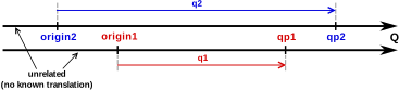
inline constexpr struct origin1 : absolute_point_origin<isq::distance> {} origin1;
inline constexpr struct origin2 : absolute_point_origin<isq::distance> {} origin2;

quantity_point qp1 = origin1 + 100 * m;
quantity_point qp2 = origin2 + 120 * m;

assert(qp1.quantity_from(origin1) == 100 * m);
assert(qp2.quantity_from(origin2) == 120 * m);

assert(qp1 - origin1 == 100 * m);
assert(qp2 - origin2 == 120 * m);
assert(origin1 - qp1 == -100 * m);
assert(origin2 - qp2 == -120 * m);

// assert(qp2 - qp1 == 20 * m);                    // Compile-time error
// assert(qp1 - origin2 == 100 * m);               // Compile-time error
// assert(qp2 - origin1 == 120 * m);               // Compile-time error
// assert(qp2.quantity_from(qp1) == 20 * m);       // Compile-time error
// assert(qp1.quantity_from(origin2) == 100 * m);  // Compile-time error
// assert(qp2.quantity_from(origin1) == 120 * m);  // Compile-time error

Relative Point origin

We often do not have only one ultimate "zero" point when we measure things. Often, we have one common scale, but we measure various quantities relative to different points and expect those points to be compatible. There are many examples here, but probably the most common are temperatures, timestamps, and altitudes.

For such cases, relative point origins should be used:

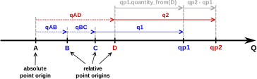
inline constexpr struct A : absolute_point_origin<isq::distance> {} A;
inline constexpr struct B : relative_point_origin<A + 10 * m> {} B;
inline constexpr struct C : relative_point_origin<B + 10 * m> {} C;
inline constexpr struct D : relative_point_origin<A + 30 * m> {} D;

quantity_point qp1 = C + 100 * m;
quantity_point qp2 = D + 120 * m;

assert(qp1.quantity_ref_from(qp1.point_origin) == 100 * m);
assert(qp2.quantity_ref_from(qp2.point_origin) == 120 * m);

assert(qp2.quantity_from(qp1) == 30 * m);
assert(qp1.quantity_from(qp2) == -30 * m);
assert(qp2 - qp1 == 30 * m);
assert(qp1 - qp2 == -30 * m);

assert(qp1.quantity_from(A) == 120 * m);
assert(qp1.quantity_from(B) == 110 * m);
assert(qp1.quantity_from(C) == 100 * m);
assert(qp1.quantity_from(D) == 90 * m);
assert(qp1 - A == 120 * m);
assert(qp1 - B == 110 * m);
assert(qp1 - C == 100 * m);
assert(qp1 - D == 90 * m);

assert(qp2.quantity_from(A) == 150 * m);
assert(qp2.quantity_from(B) == 140 * m);
assert(qp2.quantity_from(C) == 130 * m);
assert(qp2.quantity_from(D) == 120 * m);
assert(qp2 - A == 150 * m);
assert(qp2 - B == 140 * m);
assert(qp2 - C == 130 * m);
assert(qp2 - D == 120 * m);

assert(B - A == 10 * m);
assert(C - A == 20 * m);
assert(D - A == 30 * m);
assert(D - C == 10 * m);

assert(B - B == 0 * m);
// assert(A - A == 0 * m);  // Compile-time error

Note

Even though we can't subtract two absolute point origins from each other, it is possible to subtract relative ones or relative and absolute ones.

Converting between different representations of the same point

As we might represent the same point with displacement vectors from various origins, the library provides facilities to convert the same point to the quantity_point class templates expressed in terms of different origins.

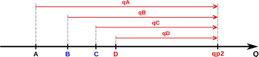
For this purpose, we can use either:

• A converting constructor:

  quantity_point<si::metre, C> qp2C = qp2;  // implicit — safe conversion within the same root
  assert(qp2C.quantity_ref_from(qp2C.point_origin) == 130 * m);
  

• A dedicated conversion interface:

  quantity_point qp2B = qp2.point_for(B);
  quantity_point qp2A = qp2.point_for(A);
  
  assert(qp2B.quantity_ref_from(qp2B.point_origin) == 140 * m);
  assert(qp2A.quantity_ref_from(qp2A.point_origin) == 150 * m);
  

It is important to understand that all such translations still describe exactly the same point (e.g., all of them compare equal):

assert(qp2 == qp2C);
assert(qp2 == qp2B);
assert(qp2 == qp2A);

Important

Between origins sharing the same absolute_point_origin root, the converting constructor may be implicit (when the quantity types are safely convertible). To convert across two independent absolute_point_origin types, a frame projection must be registered first. The constructor then works but is always explicit (no runtime arguments; use .point_for(origin, args...) when extra data is needed):

// Requires mp_units::frame_projection<sea_level, ocean_surface> to be defined:
quantity_point<si::metre, ocean_surface> depth{altitude};  // always explicit

Frame projections between independent origins

relative_point_origin handles compile-time offsets within a single origin tree. Some conversions cannot be expressed that way:

• Axis-inverting transformations — altitude ↔ depth: the physical magnitude is the same but the axis direction flips (depth = −altitude).
• Formula-based conversions — geometric azimuth ↔ bearing: bearing = 90° − azimuth involves negation, which is not a pure offset.
• Runtime-parameter conversions — world frame ↔ camera frame: the transformation depends on calibration data that is not known at compile time.

The frame_projection customization point bridges pairs of absolute_point_origin values with user-supplied callables. The primary template is intentionally left as undefined, so that the library can detect whether a user specialization exists for a given pair:

Property	relative_point_origin	frame_projection
Transformation location	Compile time (NTTP)	Runtime (callable specialization)
Rep-type requirement	Structural type	No restriction
Automatic inverse	Yes	No — both directions must be explicit
Compile-time chain discovery	Yes (origin-tree walk)	No — only direct pairs connected
Runtime parameters	No	Yes — extra point_for args forwarded to the functor
Suitable for	Celsius↔Kelvin, epoch shifts	Axis inversions, camera calibration

Defining a projection

Specialize frame_projection for each (From, To) pair. The specialization must be a callable invocable as:

frame_projection<From, To>(quantity_point_at_From, extra_args...) -> quantity_point_at_To

inline constexpr struct sea_level : absolute_point_origin<isq::altitude> {} sea_level;
inline constexpr struct ocean_surface : absolute_point_origin<isq::altitude> {} ocean_surface;

template<>
inline constexpr auto mp_units::frame_projection<sea_level, ocean_surface> =
    [](QuantityPointOf<isq::altitude> auto qp) {
        return ocean_surface - qp.quantity_from(sea_level);
    };

// The inverse must be provided explicitly — the library never derives it automatically:
template<>
inline constexpr auto mp_units::frame_projection<ocean_surface, sea_level> =
    [](QuantityPointOf<isq::altitude> auto qp) {
        return sea_level - qp.quantity_from(ocean_surface);
    };

Using point_for with a frame projection

Call point_for exactly as you would for same-origin conversions:

quantity_point altitude = sea_level + (-100. * m);            // 100 m below sea level
quantity_point depth    = altitude.point_for(ocean_surface);  // depth = 100 m (positive downward)
quantity_point alt2     = depth.point_for(sea_level);         // altitude = −100 m

If the requested origin is a relative_point_origin whose absolute root can be reached via a frame_projection, the library first projects to that absolute root and then walks down the origin tree automatically:

// shallow_water is defined 10 m "below" ocean_surface in the depth frame
inline constexpr struct shallow_water :
    relative_point_origin<ocean_surface + 10. * isq::height[m]> {} shallow_water;

quantity_point from_shallow = altitude.point_for(shallow_water);
// Steps: sea_level → ocean_surface (depth 100 m), walk-down: 100 − 10 = 90 m from shallow_water

Explicit constructor as an alternative

When no runtime arguments are needed, the explicit quantity_point constructor is a compact alternative to point_for — useful when you are already spelling out the destination type:

quantity_point<isq::altitude[m], ocean_surface> depth{altitude};
// equivalent to: altitude.point_for(ocean_surface)

The constructor invokes the same registered frame_projection internally. It is always explicit — implicit conversion across independent origins is never permitted.

Use .point_for() when extra runtime arguments must be forwarded to the projection functor (see below), or when you prefer to let the compiler deduce the destination type.

Runtime arguments

Any extra arguments passed to point_for are forwarded to the projection functor, enabling runtime-parameter-dependent transformations:

struct CameraCalibration { double R[3][3]; double t[3]; };

template<>
inline constexpr auto mp_units::frame_projection<world_frame, camera_frame> =
    [](QuantityPointOf<isq::length> auto qp, const CameraCalibration& cal) {
        return camera_frame + forward_transform(cal, qp.quantity_from(world_frame));
    };

// Different call sites supply different calibrations — no global state required:
CameraCalibration cal = load_calibration("cam.json");
quantity_point cam_pt = world_pt.point_for(camera_frame, cal);

Important

• Both directions must be explicit. The library never derives an inverse automatically.
• Chain walks within a frame are automatic. Projecting to an absolute_point_origin whose tree contains the requested relative_point_origin triggers the compile-time walk-down inside point_for.
• Chains do not cross frame boundaries. Only direct (From, To) specializations are considered; multi-hop projections must be composed by the caller.

Range-Validated Quantity Points

Background reading

For a deeper discussion of the motivation, design trade-offs, and open questions, see the blog article Range-Validated Quantity Points.

In many domains, quantity points must stay within specific bounds. For example:

• Geographic coordinates: latitude ∈ [-90°, 90°], longitude ∈ [-180°, 180°)
• Temperature sensors: operating range [−40°C, 85°C]
• Control systems: valid input range [0, 100] units

The library provides six overflow policies that can be passed as template parameters to point origins. These policies enforce bounds during construction, unit conversion, and arithmetic operations.

Production Use Case: Geographic Coordinate Systems

This feature was specifically designed to support production requirements for geographic/navigation systems, where different angle types require different wrapping behaviors:

• Latitude (symmetric): reflects at ±90° boundaries (can't go past poles)
• Longitude (mirrored): wraps circularly at -180° to +180°
• Elevation (symmetric): reflects at ±90° like latitude
• Geometric Azimuth (mirrored): 0° = East, counter-clockwise, wraps [-180°, 180°)
• Heading (mirrored): 0° = North, counter-clockwise, wraps [-180°, 180°)
  • Conversion: heading = geometric_azimuth - 90° (simple offset)
  • Uses relative_point_origin<east + delta<geometric_azimuth[degree]>(-90.)>
• Bearing (mirrored): 0° = North, clockwise, wraps [-180°, 180°)
  • Conversion: bearing = 90° - geometric_azimuth (involves negation)
  • Cannot use relative_point_origin (requires separate absolute_point_origin)
  • Use frame_projection<north_cw, east> / frame_projection<east, north_cw> — see Frame projections between independent origins

These requirements came from companies working with coordinate reference systems (CRS), navigation, and geodesy. See the complete discussion in GitHub #782.

Key Insight: relative_point_origin can only model offset transformations (addition/subtraction). Transformations involving negation or sign flips (like bearing ↔ azimuth) require separate absolute_point_origin types connected via frame_projection. This ensures type safety while allowing the framework to handle coordinate transformations automatically.

Type Safety with is_kind: All geographic quantity specs use is_kind to prevent accidental mixing of different angle types (e.g., latitude + longitude, bearing + heading). This requires explicit conversion when using trigonometric functions:

// Convert to plain angular_measure for trig functions
const quantity<angular_measure> lat_angle = isq::angular_measure(lat.quantity_from(geographic::equator));
const quantity result = sin(lat_angle);  // Works with angular_measure

The current framework handles all wrapping schemes and coordinate transformations expressible as offsets. Advanced geodetic calculations (ellipsoid parameters, distance formulas for WGS84, etc.) require additional domain-specific extensions beyond the core library. For a complete working example, see geographic.h and the UAV: Multiple Altitude Reference Systems example, which demonstrates multiple point origins, bounds checking policies, overflow handling, and coordinate reference conversions.

Available Overflow Policies

A bounds policy has min and/or max data members, which declare its range. The library finds the policy among the template arguments of an origin by these members. It reports them through quantity_point::min() and max() and through std::numeric_limits, and it compares them in the nesting check described under Hierarchical bounds validation below.

The return type of the policy's operator() sets its kind:

• A checking policy has the signature bool operator()(const V& v) const. It tells whether v lies in its domain. The value is stored unchanged, and the library reports a rejected one as the note below the table describes.
• An adjusting policy has the signature V operator()(V v) const and returns the value to store.

A policy whose operator() returns anything else, even a type convertible to bool, doesn't compile.

A plain quantity given as min or max is included in the range. exclusive_bound marks an end as excluded:

check_in_range{0 * deg, exclusive_bound{360 * deg}}  // [0°, 360°)
check_in_range{exclusive_bound{0 * m}, 100 * m}      // (0 m, 100 m]

check_in_range accepts exclusive_bound at either end. wrap_to_range excludes its maximum anyway, so it takes the maximum plain or as exclusive_bound. It rejects an excluded minimum, because a wrapped value can take that value. clamp_to_range and reflect_in_range reject exclusive_bound at compile time, since an excluded end leaves them no value to clamp or reflect to. No quantity_point::min() or max() is offered for an excluded end, including the maximum of wrap_to_range, and neither are the matching std::numeric_limits members.

Policy	Behavior	Error Handling	Use Case
check_in_range	Tests whether the value lies between min and max	Depends on rep type	Bounds checking with customizable error behavior
clamp_to_range	Clamps to nearest boundary: clamp(value, min, max)	Silent correction	Saturating arithmetic, sensor limits, UI controls
wrap_to_range	Wraps circularly to [min, max): modulo arithmetic	Value transformation	Periodic quantities (angles, time-of-day, longitude)
reflect_in_range	Reflects at boundaries (like a bouncing ball)	Value transformation	Geographic elevation angle, physical boundaries
check_non_negative	Tests whether the value is zero or positive	Depends on rep type	Inherently non-negative quantities (length, mass)
clamp_non_negative	Clamps negative values to zero	Silent correction	FP rounding noise in non-negative domains

check_in_range and check_non_negative reject NaN. wrap_to_range and reflect_in_range reduce a finite value of any magnitude into the range and return NaN for an infinite or NaN input.

Important

The four bounded-range policies (check_in_range, clamp_to_range, wrap_to_range, reflect_in_range) have both min and max data members. check_non_negative and clamp_non_negative are halfline policies with no upper bound and therefore do not expose max. See the std::numeric_limits note below for details.

Error behavior of checking policies

What happens to a value that a checking policy such as check_in_range rejects depends on the representation type:

• If the rep has a constraint_violation_handler specialization (e.g. constrained<double, throw_policy>), the operation has a wide contract. The library calls the handler's on_violation() in every build mode. The handler may throw, terminate, or log and return. If it returns, the value is stored unchanged.
• Otherwise, the operation has a narrow contract. The value must lie within the bounds as a precondition of construction of a point from a value, of the converting constructors (including unit and origin conversion), and of ++, --, +=, and -=. The library declares this precondition with C++26 pre where it can and otherwise checks it in the function body with the configured contract backend, if any. How a violation is handled follows the contract configuration of the build.

To test a value before storing it, use is_within_bounds or try_make, described in Validating Untrusted Values.

See Tutorial: Custom Contract Handlers for a step-by-step guide to implementing custom error policies, or How to: Ensure Ultimate Safety for a complete example of combining check_in_range with constrained rep types.

Example Usage

// Define quantity specifications and origins
inline constexpr struct geo_latitude : quantity_spec<isq::angular_measure> {} geo_latitude;
inline constexpr struct geo_longitude : quantity_spec<isq::angular_measure> {} geo_longitude;

inline constexpr struct equator :
    absolute_point_origin<geo_latitude, reflect_in_range{-90 * si::degree, 90 * si::degree}> {} equator;
inline constexpr struct prime_meridian :
    absolute_point_origin<geo_longitude, wrap_to_range{-180 * si::degree, 180 * si::degree}> {} prime_meridian;

// Define bounded quantity point types
template<typename T = double> using latitude = quantity_point<si::degree, equator, T>;
template<typename T = double> using longitude = quantity_point<si::degree, prime_meridian, T>;

void example()
{
  latitude lat = equator + 45.0 * deg;           // Valid: within [-90, 90]
  lat = equator + 95.0 * deg;                    // Reflects to 85° (reflect_in_range mirrors at boundary)

  longitude lon = prime_meridian + 270.0 * deg;  // Wraps to -90° (wrap_to_range treats range as circular)
  lon += 200.0 * deg;                            // Result wraps: -90 + 200 = 110°
}

Simplified

True geodetic latitude reflection also requires shifting longitude by 180° (crossing a pole puts you on the opposite side of the globe).

How It Works

Bounds are enforced at these points:

1. Construction from a quantity: quantity_point{value * unit, origin}
2. Unit conversion: qp.in(other_unit), qp.in(other_unit, policy)
3. Arithmetic operations: operator+=, operator-=, operator++, operator--
4. Origin conversion: qp.point_for(new_origin)

After each mutation the library transparently applies the bounds policy specified on the origin.

Bounds the Point Can Hold

A policy compares a value with its bounds in the value's own type. Each bound therefore has to be exactly representable in the point's quantity type (for a floating-point representation, in the bound's own unit). Otherwise the policy would compare against a rounded bound. A point whose quantity type can't hold a bound offers no constructor from a quantity, no is_within_bounds, and no try_make:

inline constexpr struct tape_start :
    absolute_point_origin<isq::length, check_in_range{0.1 * m, 10. * m}> {} tape_start;
inline constexpr struct tape_start_f :
    absolute_point_origin<isq::length, check_in_range{0.1f * m, 10.f * m}> {} tape_start_f;

quantity_point<isq::length[m], tape_start> p1{0.5 * m, tape_start};             // OK
quantity_point<isq::length[m], tape_start_f, float> p2{0.5f * m, tape_start_f};  // OK
// quantity_point<isq::length[m], tape_start, float> p3{0.5f * m, tape_start};   // ❌

p3 doesn't compile because the double value of 0.1 isn't a float value. A float point needs an origin with float bounds, such as tape_start_f. A bound with a small integral value, such as -90. * deg, is exact in float, which holds every integer up to 16'777'216.

With a floating-point representation, scaling a bound to the point's unit is accepted, because it can't be exact in general (0.3048 m per foot has no exact binary form).

Origin Inheritance

A relative_point_origin that defines no own bounds automatically inherits the enforcement of its nearest bounded ancestor. Bounds translate through the chain at compile time. The relative value is translated to the owning ancestor's frame and the policy is applied there. A value the policy changed is translated back, and a value it let through is stored as it was:

inline constexpr struct sea_level :
    absolute_point_origin<isq::altitude, clamp_to_range{-500 * m, 12'000 * m}> {} sea_level;

// Relative origin — no own bounds; inherits clamping from sea_level.
inline constexpr struct airport_elevation :
    relative_point_origin<sea_level + 200 * m> {} airport_elevation;

// 11'900 m above airport = 12'100 m MSL → exceeds 12'000 m cap → clamped to 11'800 m from airport.
quantity_point takeoff = airport_elevation + 11'900.0 * m;

This applies to all bound policies — including the check_non_negative bounds that are automatically attached to natural_point_origin of a non-negative quantity spec. A relative origin above the ground floor may therefore hold negative values, as long as the absolute position stays ≥ 0:

inline constexpr struct height_spec : quantity_spec<isq::height> {} height_spec;

// natural_point_origin<height_spec> auto-gets check_non_negative (isq::height is non_negative).
inline constexpr struct average_height_origin :
    relative_point_origin<natural_point_origin<height_spec> + 1700.0 * m> {} average_height_origin;

// −1500 m relative = 200 m absolute (≥ 0) → valid, unchanged.
quantity_point low = average_height_origin - 1500.0 * m;

// −1701 m relative = −1 m absolute → check_non_negative fires.
// quantity_point bad = average_height_origin - 1701.0 * m;  // ❌

A point is translated into the frame of its bounded ancestor by the offset to that ancestor. With an integral representation, the point's quantity type must hold that offset exactly, as it must hold the bounds (see Bounds the Point Can Hold): an int point measured from an origin 0.5 m above its bounded ancestor, or an int kilometre point 1500 m above it, is rejected. With a floating-point representation, rounding the offset is accepted.

When a relative_point_origin defines its own bounds, they are additionally checked at compile time to nest within the bounds of the nearest bounded origin above it (see the Hierarchical bounds validation note in the Custom Policies section below).

std::numeric_limits integration

When a quantity_point has a bounds policy on its origin, the std::numeric_limits specialization automatically reflects the constrained bounds:

// prime_meridian defined with wrap_to_range{-180 * deg, 180 * deg}
using longitude = quantity_point<geo_longitude[deg], prime_meridian>;

quantity_point lon_min = std::numeric_limits<longitude>::min();  // prime_meridian - 180°
// auto lon_max = std::numeric_limits<longitude>::max();         // ❌ 180° is excluded

This works because the policy struct exposes public min and max data members, which quantity_point::min() and max() access to provide meaningful bounds. A relative origin without bounds of its own reports those of its nearest bounded ancestor, translated into its frame. With a floating-point representation the translation rounds, so min() and max() report the lowest and highest values that ancestor's bounds accept, which can differ from the translated bound by the rounding of each offset. Without a bounds policy, std::numeric_limits delegates to the representation type's limits.

Validating Untrusted Values

A value read from a sensor, a bus, or persistent storage often has to be rejected without stopping the program. Catching the violation works only when the representation throws, and code built without exceptions has nothing to catch.

The static member function is_within_bounds tells whether constructing the point from the same arguments would satisfy the bounds. It doesn't construct the point:

inline constexpr struct trim_zero :
    absolute_point_origin<isq::angular_measure, check_in_range{-10. * deg, 10. * deg}> {} trim_zero;

using trim_angle =
    quantity_point<si::degree, trim_zero, utility::constrained<double, utility::terminate_policy>>;

std::optional<trim_angle> make_trim(quantity<si::degree> raw)
{
  if (!trim_angle::is_within_bounds(raw, trim_zero)) return std::nullopt;
  return trim_angle{raw, trim_zero};
}

Where <expected> is available (C++23), the static member function try_make does the same in one call and returns a rejection as an error value:

std::expected<trim_angle, bounds_violation> try_make_trim(quantity<si::degree> raw)
{
  return trim_angle::try_make(raw, trim_zero);
}

A rejected value is never passed to the constructor. The representation's violation handler is not called and no precondition is violated, so both functions work in code built with -fno-exceptions and under any contract evaluation semantic.

The test follows construction in two steps:

• The value is first converted to the point's quantity type, as the constructor does. An integral narrowing conversion therefore happens before the test.
• The value is tested against the bounds of the point's origin. For a relative_point_origin without bounds of its own, the value is translated into the frame of its nearest bounded ancestor and tested against that ancestor's bounds. The compile-time nesting check (see Hierarchical bounds validation below) makes testing those bounds enough.

The conversion and the translation into an ancestor's frame are done by the representation. A representation that checks its own arithmetic, such as safe_int, can still throw or terminate there.

Both functions are available when the point's bounds are enforced by a checking policy, a user-defined one included, and for a point without bounds, where is_within_bounds always returns true. They call the same predicate that construction calls. The library's adjusting policies replace an out-of-range value instead of rejecting it, so neither function is offered for them.

Custom Policies (One-Sided Bounds)

The library ships two built-in one-sided halfline policies for [0, +∞) domains: check_non_negative (rejects a negative or NaN value) and clamp_non_negative (silently clamps negative values to zero). These are automatically applied to any quantity_point whose origin is a natural_point_origin of a non-negative quantity spec (such as isq::length, isq::mass, or isq::duration).

For other one-sided constraints, you can create a fully custom policy. This one is an adjusting policy:

template<Quantity Q>
struct clamp_bottom {
  Q min;  // Public member enables std::numeric_limits support

  template<Quantity V>
  constexpr V operator()(V v) const { return v < min ? min : v; }
};

// Usage: hydraulic system with minimum operating pressure
inline constexpr struct atmospheric_pressure :
    absolute_point_origin<isq::pressure, clamp_bottom{1000 * si::kilo<si::pascal>}> {} atmospheric_pressure;

using hydraulic_pressure = quantity_point<si::kilo<si::pascal>, atmospheric_pressure>;
hydraulic_pressure p1 = atmospheric_pressure + 2000 * kPa;  // OK: 2000 kPa
hydraulic_pressure p2 = atmospheric_pressure + 500 * kPa;   // Clamped to 1000 kPa (min operating pressure)

A range with an excluded end doesn't need a custom policy. A heading in [0°, 360°) is check_in_range with an exclusive_bound maximum:

inline constexpr struct heading_zero :
    absolute_point_origin<isq::angular_measure, check_in_range{0. * deg, exclusive_bound{360. * deg}}> {} heading_zero;

A custom checking policy is for a domain that is not an interval. A transmitter, for example, may only be tuned within its allowed bands, here from 2.4 GHz to 2.4835 GHz and from 5.725 GHz to 5.875 GHz:

template<Quantity Q>
struct check_in_bands {
  Q min;              // first band: [min, first_band_max]
  Q first_band_max;
  Q second_band_min;  // second band: [second_band_min, max]
  Q max;

  template<Quantity V>
  constexpr bool operator()(const V& v) const
  {
    return (v >= V{min} && v <= V{first_band_max}) || (v >= V{second_band_min} && v <= V{max});
  }
};

inline constexpr struct tuning_zero :
    absolute_point_origin<isq::frequency, check_in_bands{2.4 * GHz, 2.4835 * GHz, 5.725 * GHz, 5.875 * GHz}> {} tuning_zero;

using tx_frequency = quantity_point<isq::frequency[GHz], tuning_zero>;

static_assert(tx_frequency::is_within_bounds(2.45 * GHz, tuning_zero));
static_assert(!tx_frequency::is_within_bounds(3. * GHz, tuning_zero));

Its min and max declare the outer ends of the domain, which quantity_point::min() and max() report.

Hierarchical bounds validation

When a relative_point_origin defines bounds, the library enforces at compile time that they fit within the bounds of its nearest bounded ancestor (after translating to that ancestor's reference frame). Origins without bounds of their own between the two are skipped. If that ancestor has a lower or an upper bound, the child must declare that bound too. The bounds are compared by value and by exclusivity. Where the ancestor excludes an end and the child includes it, the child's end must lie strictly inside the ancestor's range. A child of a wrap_to_range ancestor must thus end strictly below the ancestor's maximum, unless it excludes its own maximum too. A user-defined checking policy is compared by its min and max as well, and its predicate is not consulted. A value inside an origin's own bounds therefore lies between the min and max of every bounded origin above it, up to rounding with floating-point offsets. Each floating-point offset in the chain rounds, so a value at the edge of a child's range can end up one ulp outside an ancestor's range several levels up.

Defining the origin or naming a point type doesn't trigger the check. It fires when the origin's bounds are first used, for example when a point is constructed from a value, in arithmetic, in is_within_bounds or try_make, or in min() and max().

This hierarchical validation ensures semantic correctness: if you model origin B as relative to origin A, and A has operational constraints, then B inheriting those constraints is physically and logically appropriate (e.g., a room's temperature range shouldn't exceed the building HVAC system's capability, a drone's altitude above launch point shouldn't exceed airspace authorization limits).

Absolute origin bounds represent physical constraints (e.g., temperature can't go below absolute zero) and are always enforced—this is non-negotiable.

Relative origin bounds hierarchical enforcement represents our current design decision based on typical use cases. If you encounter scenarios where nested relative origins need independent bounds (not constrained by their parent), please share your feedback so we can evaluate adding opt-in flexibility.

Implementation reference

See geographic.h and overflow_policies.h for complete examples.

Temperature support

Support for temperature quantity points is probably one of the most common examples of relative point origins in action that we use in daily life.

The SI definition in the library provides a few predefined point origins for this purpose:

namespace si {

inline constexpr struct absolute_zero : absolute_point_origin<isq::thermodynamic_temperature> {} absolute_zero;

inline constexpr struct ice_point : relative_point_origin<point<milli<kelvin>>(273'150)}> {} ice_point;

}

namespace usc {

inline constexpr struct fahrenheit_zero :
  relative_point_origin<point<mag_ratio<5, 9> * si::degree_Celsius>(-32)> {} fahrenheit_zero;

}

The above is a great example of how point origins can be stacked on top of each other:

• usc::fahrenheit_zero is defined relative to si::ice_point
• si::ice_point is defined relative to si::absolute_zero.

Note

Notice that while stacking point origins, we can use different representation types and units for origins and a point. In the above example, the relative point origin for degree Celsius is defined in terms of si::kelvin, while the quantity point for it will use si::degree_Celsius as a unit.

The temperature point origins defined above are provided explicitly in the respective units' definitions:

namespace si {

inline constexpr struct kelvin :
    named_unit<"K", kind_of<isq::thermodynamic_temperature>, absolute_zero> {} kelvin;
inline constexpr struct degree_Celsius :
    named_unit<{u8"℃", "`C"}, kelvin, ice_point> {} degree_Celsius;

}

namespace usc {

inline constexpr struct degree_Fahrenheit :
    named_unit<{u8"℉", "`F"}, mag_ratio<5, 9> * si::degree_Celsius,
               fahrenheit_zero> {} degree_Fahrenheit;

}

As it was described above, default_point_origin(R) returns a natural_point_origin<QuantitySpec> when a unit does not provide any origin in its definition. As of today, the units of temperature are the only ones in the entire mp-units library that provide such origins.

Now, let's see how we can benefit from the above definitions. We have quite a few alternatives to choose from here. Depending on our needs or tastes, we can:

• be explicit about the unit and origin:

  quantity_point<si::degree_Celsius, si::ice_point> q1 = si::ice_point + delta<deg_C>(20.5);
  quantity_point<si::degree_Celsius, si::ice_point> q2{delta<deg_C>(20.5), si::ice_point};
  quantity_point<si::degree_Celsius, si::ice_point> q3{delta<deg_C>(20.5)};
  quantity_point<si::degree_Celsius, si::ice_point> q4 = point<deg_C>(20.5);
  

• specify a unit and use its point origin implicitly:

  quantity_point<si::degree_Celsius> q5 = si::ice_point + delta<deg_C>(20.5);
  quantity_point<si::degree_Celsius> q6{delta<deg_C>(20.5), si::ice_point};
  quantity_point<si::degree_Celsius> q7{delta<deg_C>(20.5)};
  quantity_point<si::degree_Celsius> q8 = point<deg_C>(20.5);
  

• benefit from CTAD:

  quantity_point q9 = si::ice_point + delta<deg_C>(20.5);
  quantity_point q10{delta<deg_C>(20.5), si::ice_point};
  quantity_point q11{delta<deg_C>(20.5)};
  quantity_point q12 = point<deg_C>(20.5);
  

In all of the above cases, we end up with the quantity_point of the same type and value.

To play a bit more with temperatures, we can implement a simple room AC temperature controller in the following way:

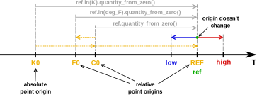
Now that the Range-Validated Quantity Points infrastructure is available, we can attach a clamp_to_range policy so the controller silently enforces the comfort band:

constexpr struct room_reference_temp :
    relative_point_origin<point<deg_C>(21), clamp_to_range{delta<deg_C>(-3), delta<deg_C>(3)}> {} room_reference_temp;
using room_temp = quantity_point<deg_C, room_reference_temp>;

constexpr auto step_delta = delta<deg_C>(0.5);
constexpr int number_of_steps = 6;

room_temp room_ref{};
room_temp room_low  = room_ref - number_of_steps * step_delta;  // −3 °C: exactly at lower bound
room_temp room_high = room_ref + number_of_steps * step_delta;  // +3 °C: exactly at upper bound

// Any attempt to exceed the ±3 °C comfort range is silently clamped
room_temp clamped = room_ref + delta<deg_C>(10.0);              // → auto-clamped to +3 °C from reference

std::println("Room reference temperature: {} ({}, {::N[.2f]})\n",
             room_ref,
             room_ref.in(usc::degree_Fahrenheit),
             room_ref.in(si::kelvin));

std::println("| {:<18} | {:^18} | {:^18} | {:^18} |",
             "Temperature delta", "Room reference", "Ice point", "Absolute zero");
std::println("|{0:=^20}|{0:=^20}|{0:=^20}|{0:=^20}|", "");

auto print_temp = [&](std::string_view label, auto v) {
  std::println("| {:<18} | {:^18} | {:^18} | {:^18:N[.2f]} |", label,
               v - room_reference_temp, (v - si::ice_point).in(deg_C), (v - si::absolute_zero).in(deg_C));
};

print_temp("Lowest", room_low);
print_temp("Default", room_ref);
print_temp("Highest", room_high);
print_temp("Clamped to max", clamped);

The above prints:

Room reference temperature: 21 ℃ (69.8 ℉, 294.15 K)

| Temperature delta  |   Room reference   |     Ice point      |   Absolute zero    |
|====================|====================|====================|====================|
| Lowest             |       -3 ℃        |       18 ℃        |     291.15 ℃      |
| Default            |        0 ℃        |       21 ℃        |     294.15 ℃      |
| Highest            |        3 ℃        |       24 ℃        |     297.15 ℃      |
| Clamped to max     |        3 ℃        |       24 ℃        |     297.15 ℃      |

Text output for Points

Text output is supported for quantity_point when its point origin equals default_point_origin(R) — the library-chosen default for the given reference.

• For references without an offset unit (e.g., quantity_point<isq::length[m]>), default_point_origin is natural_point_origin<QuantitySpec>, which represents the mathematical zero. The stored quantity is unambiguous:

  quantity_point qp{42 * m};
  std::cout << qp;  // "42 m"
  

• For references whose unit carries a built-in origin (e.g., quantity_point<deg_C>), default_point_origin is the unit's canonical reference point (si::ice_point). The output matches the conventional notation:

  quantity_point temp = point<deg_C>(20.);
  std::cout << temp;  // "20 ℃"
  

Text output is not provided when a non-default origin is used, for example:

inline constexpr struct sea_level : absolute_point_origin<isq::altitude> {} sea_level;
quantity_point<isq::altitude[m], sea_level> altitude = sea_level + 42 * m;
std::cout << altitude;  // ❌ — does not compile

The stored quantity is a displacement from a domain-specific reference whose name the library cannot know. The same numeric value can describe entirely different physical locations depending on the choice of origin — "42 m" above sea level, a mountain top, or the centre of Mars are all distinct points. Providing a meaningful text representation would require origin-aware formatting that is beyond what the library can infer from the type alone.

To print such a point, extract the displacement from a known origin explicitly and add the appropriate label so the value is unambiguous:

std::cout << altitude.quantity_ref_from(sea_level) << " AMSL";  // "42 m AMSL"

Extracting a raw numerical value from a Point

At the boundary of our program (serialization, hardware registers, a user interface) we often need the plain number stored in a point. For a point that uses default_point_origin(R), the numerical_value_in(Unit) member function returns that value directly. It is the exact inverse of the point<Unit>(value) helper and reads the point on the scale of the requested unit, re-anchoring across offset units when needed:

quantity_point temp = point<deg_C>(20.5);

double celsius = temp.numerical_value_in(deg_C);  // 20.5
double kelvin = temp.numerical_value_in(K);       // 293.65 (measured from absolute zero)

A truncating variant, numerical_value_in(Unit, policy), is provided for conversions that would otherwise be rejected as value-preserving (e.g., an integer representation scaled to a coarser unit).

Both member functions are available under exactly the same condition as text output: only when the point uses default_point_origin(R). A point with a custom origin has no unique numerical representation, so its value must be requested from an explicit origin instead:

double above_sea_level = altitude.quantity_from(sea_level).numerical_value_in(m);

The affine space is about type-safety

The following operations are not allowed in the affine space:

• adding two quantity_point objects
  • It is physically impossible to add positions of home and Denver airports.
• subtracting a quantity_point from a quantity
  • What would it mean to subtract the DEN airport location from the distance to it?
• multiplying/dividing a quantity_point with a scalar
  • What is the position of 2 * DEN airport location?
• multiplying/dividing a quantity_point with a quantity
  • What would multiplying the distance with the DEN airport location mean?
• multiplying/dividing two quantity_point objects
  • What would multiplying home and DEN airport location mean?
• mixing quantity_points of different quantity kinds
  • It is physically impossible to subtract time from length.
• mixing quantity_points of quantity types on distinct natural axes (e.g., height and width, or distance and altitude), even though their vectors widen to a common ancestor (see Quantity types and points)
  • What does subtracting a distance point to DEN airport from the Mount Everest base camp altitude mean?
• mixing quantity_points of convertible quantities but with unrelated origins
  • How do we subtract a point on our trip to CppCon measured relatively to our home location from a point measured relative to the center of the Solar System?

Important: The affine space improves safety

The usage of quantity_point and affine space types, in general, improves expressiveness and type-safety of the code we write.